
 Search
Learning | Energy & Commodity Derivatives
How to Value Power Purchase Agreements
Introductory Summary
A Power Purchase Agreement (PPA) can provide long-term revenue certainty for a renewable generator or a long-term supply arrangement for a buyer. But the economic value of a PPA is rarely determined by its fixed price alone.
For a renewable PPA, the value and risk profile can depend on the interaction between the contract terms, power prices, the generation profile of the underlying asset, market seasonality, intraday price shape and uncertainty in renewable production. A pay-as-produced PPA, for example, can leave a purchaser exposed to significant volume and shape risk even when the contract price itself appears attractive against the market forward curve.
Valuing and risk-managing these agreements therefore requires more than comparing a PPA price with a market price. The analysis needs to capture how the renewable asset is expected to produce, how power prices behave at the relevant time intervals, and how those variables may evolve together over the life of the agreement.
This article explains a practical framework for doing that analysis.
Start with the PPA Structure
Before building a valuation model, the first question is deceptively simple:
What exactly is the PPA transferring between the parties?
The answer determines which risks need to be modelled.
A PPA might be structured as a physical or financial agreement, and the volume obligation may be linked to actual production, a fixed delivery profile or the buyer’s consumption. These distinctions can materially change the risk borne by each party.
The valuation therefore needs to begin with the contractual economics rather than the modelling technique.
For a more detailed explanation of the different structures, see the What is a Power Purchase Agreement (PPA)? article.
Questions to Establish Before Valuation
A useful initial assessment asks:
- Is the PPA physical or financial?
- Is the volume Pay-as-Produced, Pay-as-Consumed, or Fixed Volume Delivery?
- What is the contract price?
- What is the term of the agreement?
- Which market and price index apply?
- How is generation measured?
- Who bears volume risk?
- Who bears price risk?
- Are there shaping, balancing or other associated costs?
- Are there contractual floors, caps or other flexibilities?
- What happens when generation differs from the expected profile?
- What risks remain after any contractual or market hedges?
These questions determine the market data, model inputs and assumptions required later in the analysis.
A PPA Is More Than a Price Risk
One of the easiest mistakes in PPA analysis is to focus on the fixed contract price and treat the agreement as though it were simply a long-dated power swap.
For a renewable PPA, the exposure can have several dimensions:
- Price risk arises because the value of generated electricity changes as market power prices move
- Volume risk arises because renewable production is uncertain
- Shape risk arises because the timing of production does not necessarily match the shape of market prices or the hedge used to manage the PPA
- Basis risk can arise where the PPA generation location, pricing index and available hedging instruments do not perfectly correspond
- Seasonal risk reflects differences in both power prices and renewable generation throughout the year
These risks interact. A wind farm may generate more electricity during a period when power prices are low. Conversely, solar generation is concentrated in daylight hours, meaning that a simple flat baseload hedge may not reproduce the actual economic exposure particularly well.
The important point is that the risk is created by the interaction between price and production, rather than by either variable in isolation.
The Core Building Blocks of a PPA Valuation
A robust PPA analysis brings several important components together:
- Power price curves
- Intraday and seasonal price shaping
- Renewable generation modelling
- Stochastic simulation
- Portfolio and hedge analysis
Each component answers a different question.
The forward curve provides the market’s current pricing reference. Historical analysis adds the detail that is not directly observable in longer-dated market quotes. Renewable production modelling describes how much power the asset may generate. Stochastic simulation then combines these elements to explore the range of possible future outcomes.
Build the Power Price Representation
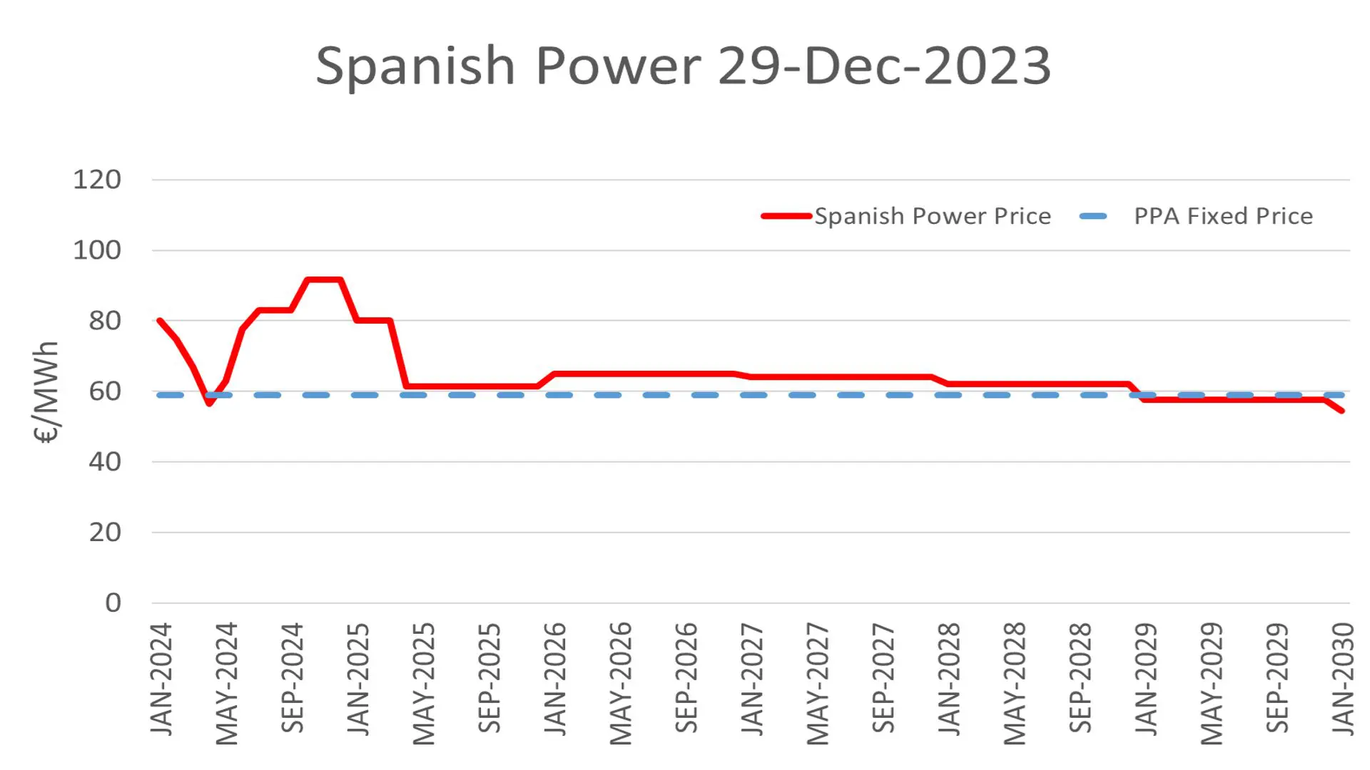
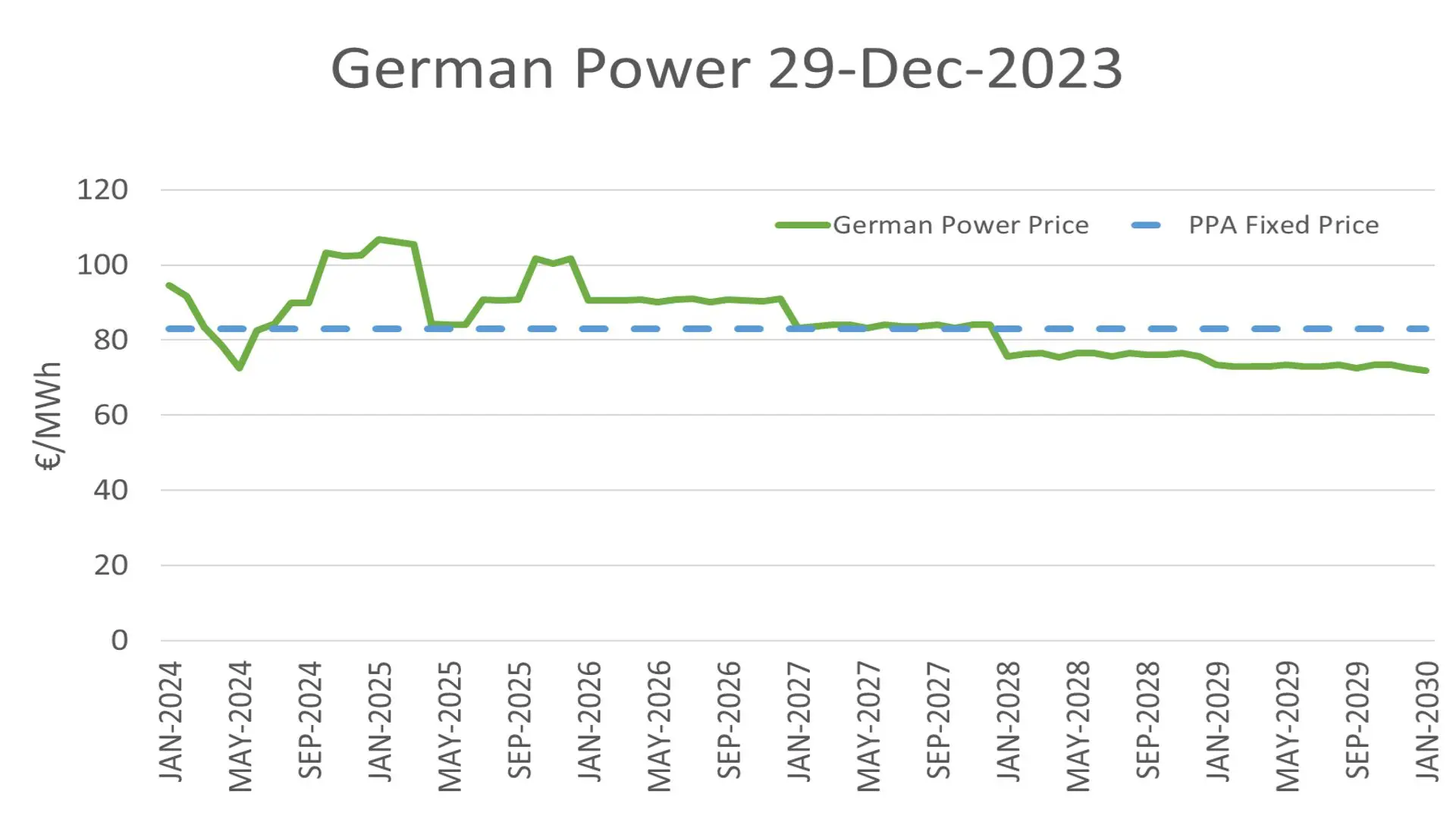
The starting point is normally the market forward curve for the relevant power market. However, the quoted forward market often does not provide the hourly detail required to value a renewable PPA.
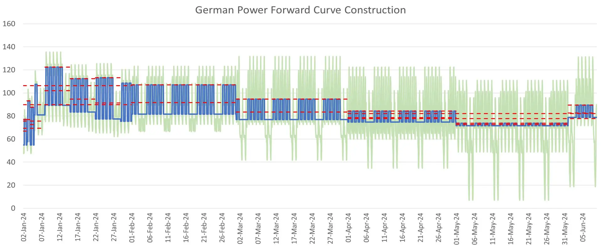
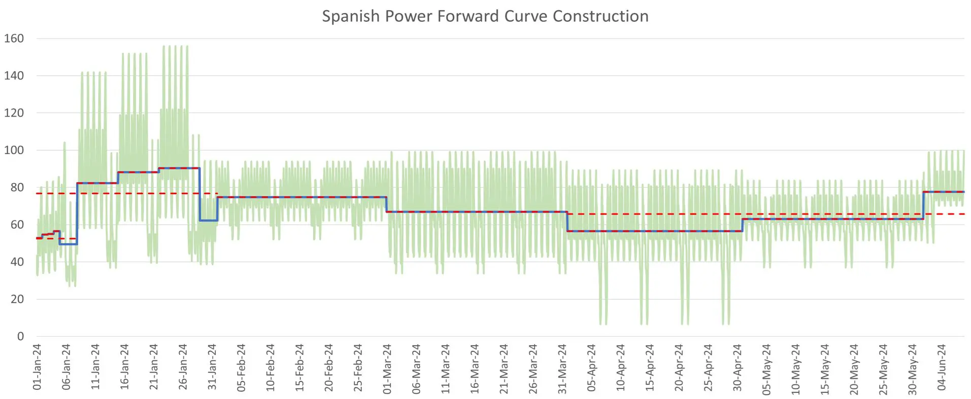
For example, a market may provide base and peak contracts across different maturities. These overlapping market quotes need to be transformed into a consistent representation of the forward market before the hourly characteristics of the PPA can be incorporated.
For more detail on constructing forward curves, see How to Build an Energy Forward Curve.
Why Hourly Shape Matters
Renewable production is inherently time-dependent.
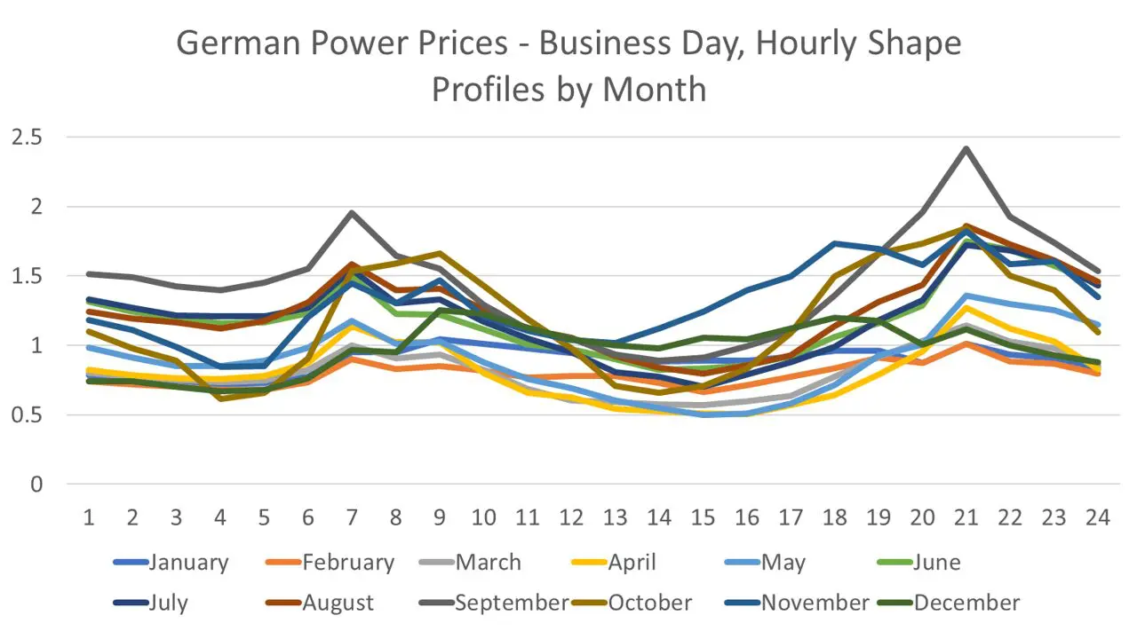
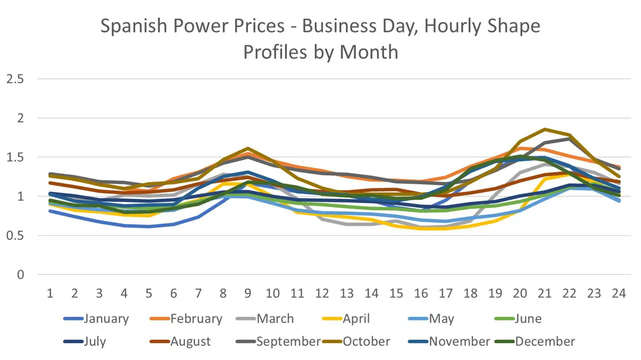
A solar asset produces during daylight hours, with production changing through the year. Wind generation has a different profile and generally does not exhibit the same deterministic intraday pattern. If the valuation uses only a flat annual or monthly power price, it can miss an important part of the economics.
Historical power-price data can therefore be analysed to identify patterns such as:
- hourly price shapes;
- weekday versus weekend profiles;
- monthly or seasonal differences;
- peak and off-peak behaviour; and
- other market-specific patterns.
The appropriate level of detail depends on the purpose of the analysis.
A model might distinguish business and non-business days, for example, or use monthly shaping. In other circumstances, it may be appropriate to use more granular profiles such as individual weekdays or other time buckets.
There is no universally correct calibration breakdown. The objective is to use a representation that captures the characteristics relevant to the PPA without introducing unnecessary complexity.
From Market Quotes to an Hourly Forward Curve
The distinction between a quoted forward curve and an hourly forward curve is particularly important for renewable PPAs.
Suppose the market provides base and peak prices. These prices can be used to construct a daily forward curve consistent with the observable market. Historical shaping parameters can then be applied to that curve to produce hourly prices.
The shaping parameters should be normalised so that aggregating the resulting hourly prices back to the relevant market periods remains consistent with the quoted forward prices.
This gives the analysis two useful properties:
- market consistency, because the shaped curve remains consistent with observable market quotes; and
- granularity, because the resulting curve contains the hourly information required to analyse renewable generation.
Where only base prices are available, shaping becomes even more important because there is less intraday information embedded directly in the market quotes.
This is one reason why forward curve construction and shaping are not merely data-preparation exercises. They can materially influence the valuation and risk results.
Model the Renewable Generation Profile
The other half of the PPA valuation is the renewable asset itself.
For a wind PPA, this means modelling wind speeds and converting them into electricity production. For a solar PPA, the corresponding variables include solar irradiance and the relationship between irradiance and generation.
The analysis therefore needs to capture both the availability of the underlying renewable resource and the conversion from that resource into power output.
Wind Generation
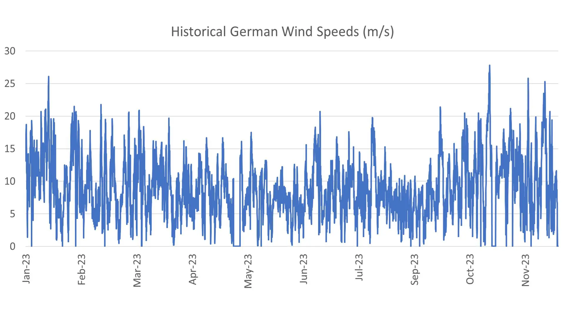
Historical wind-speed data can be analysed to establish characteristics such as:
- seasonal behaviour;
- variability;
- frequency and magnitude of spikes;
- hourly characteristics; and
- longer-term changes in the observed distribution.
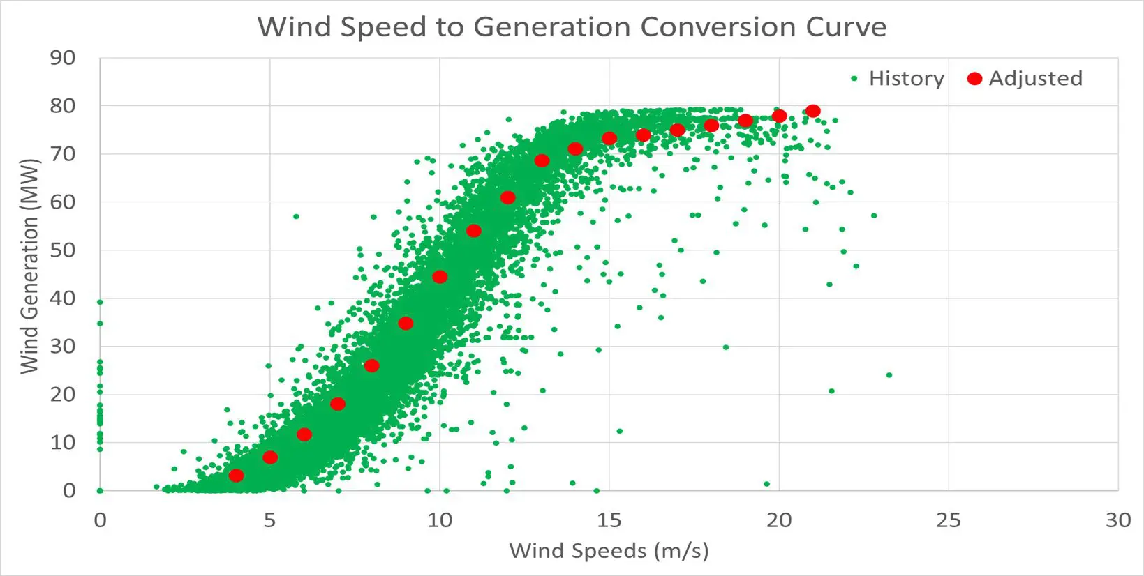
The wind-speed series can then be transformed into expected generation using an appropriate conversion relationship, commonly represented by a power curve or S-curve. This relationship maps wind speed to electricity output.
Where suitable historical wind-speed and generation data are available, participants can calibrate a relationship specific to the asset or data set being analysed.
Solar Generation
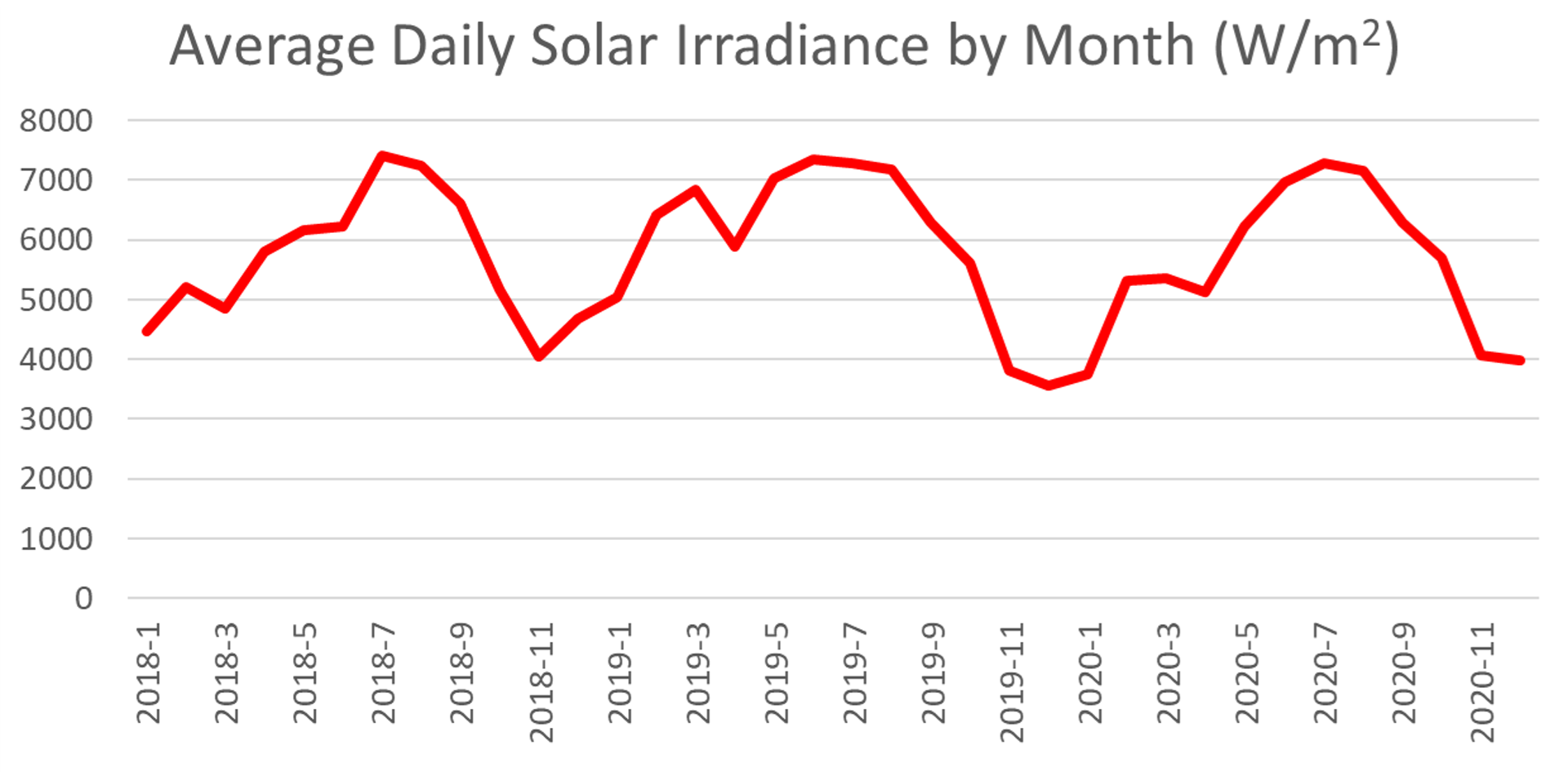
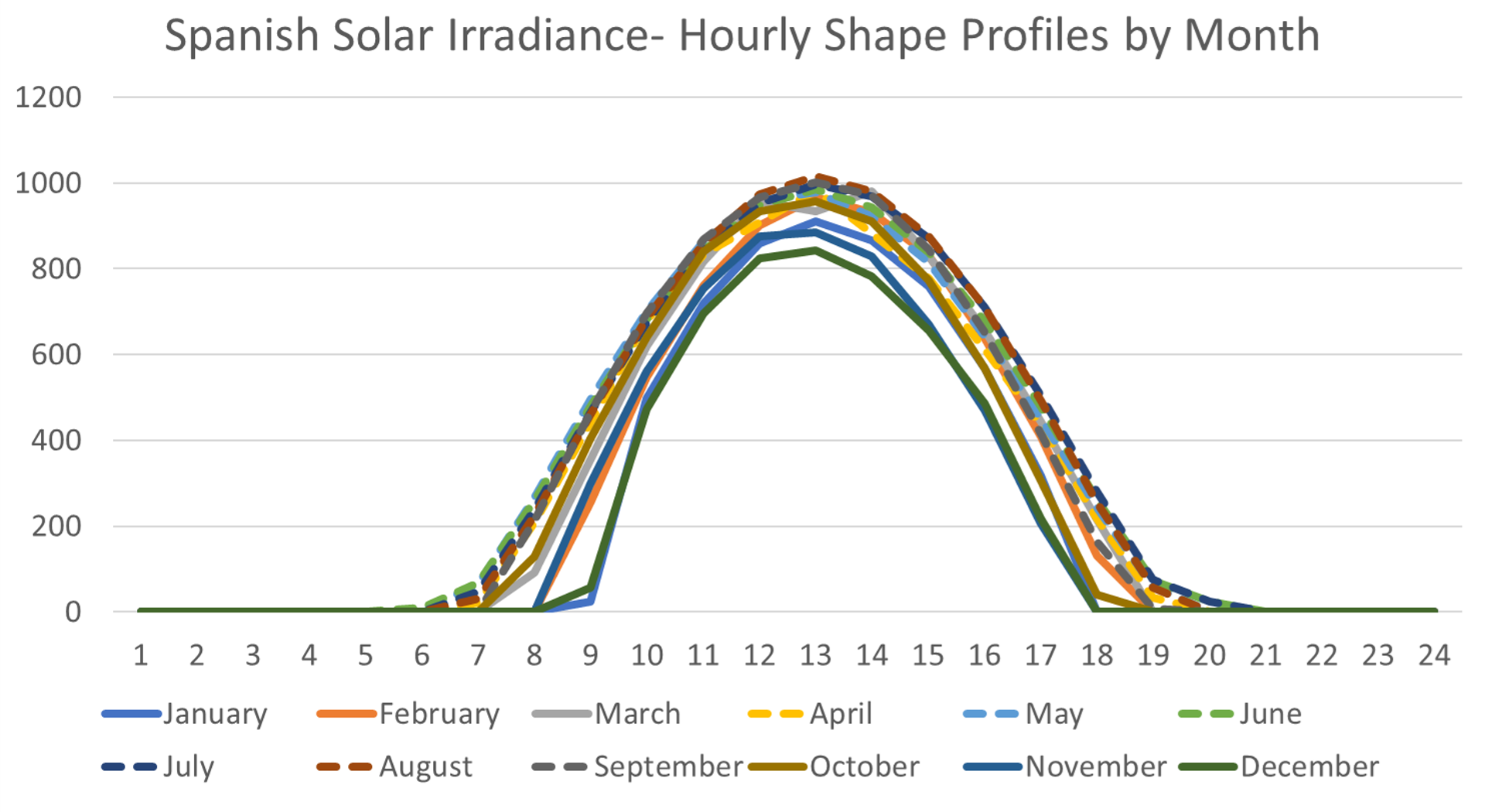
Solar irradiance presents a somewhat different modelling challenge.
There is a strong deterministic component to solar production. There is no solar generation during the night, and the number and timing of daylight hours changes through the year. A calibration that simply averages historical observations across all months can therefore produce unrealistic results.
The modelling process should recognise these known structural characteristics while still representing the uncertainty around actual production.
Calibration Is Part Science, Part Judgement
Calibration is not simply a matter of feeding historical observations into a statistical routine. The statistical process may be highly systematic: a model is selected, historical observations are supplied, and parameters such as volatility, mean reversion or jump characteristics are estimated.
The more difficult question however, is whether the historical period chosen remains representative of the market being modelled.
For example, a wind-speed history might show substantially more variability and spikes in its most recent year than in the preceding years. A modeller could choose to calibrate heavily towards that recent behaviour because it may be considered more representative of current conditions. Alternatively, the recent period could be treated as an unusual observation and a longer history could be used.
This judgement becomes particularly important for long-dated PPAs. A calibration that appears appropriate today cannot simply be assumed to remain appropriate for the entire life of a 10 or 15-year agreement.
For a broader discussion of model calibration, see What is Calibration Risk?
Capture the Joint Behaviour of Price and Generation
The valuation becomes more interesting when the power-price and renewable-generation models are brought together.
A simple approach might represent their relationship using correlation.
Correlation can be useful, but it may not fully capture the economics of renewable-heavy power markets. For example, increasing wind generation in a particular region can contribute to increased supply and potentially put downward pressure on power prices.
If the relationship between wind generation and power prices is expected to be economically meaningful, simply imposing a historical correlation may not be sufficient. More sophisticated approaches can introduce a functional or transformation relationship between the variables.
The broader principle is important:
If two variables interact economically, modelling them as correlated but otherwise independent processes may fail to capture the relationship that matters most to the valuation.
This is particularly relevant when analysing long-dated renewable portfolios, where the structure of the power market itself may evolve as renewable penetration increases.
For more on relationships between market variables, see What is Correlation Risk?
Use Stochastic Simulation to Value the PPA
Once the market and generation models have been calibrated, they can be used to generate simulations of future outcomes.
For each simulated scenario, the model produces a path for the relevant power prices and renewable generation levels. These are combined with the contractual terms of the PPA to calculate the resulting cash flows.
The process can be thought of as:
Simulate market and generation variables → calculate hourly PPA cash flows → aggregate cash flows → discount to the valuation date
Repeating this process many times produces a distribution of possible PPA values or cash flows rather than a single deterministic number.
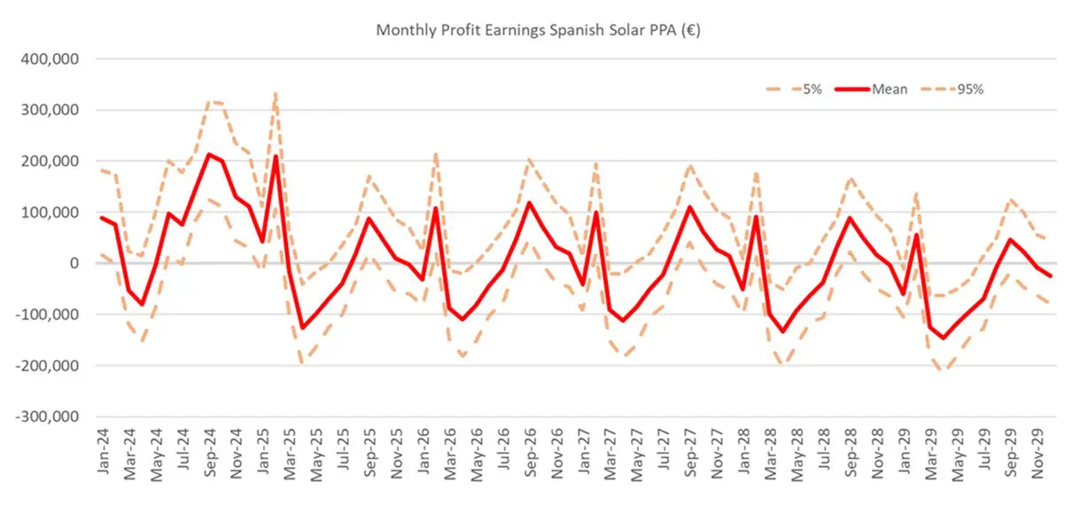
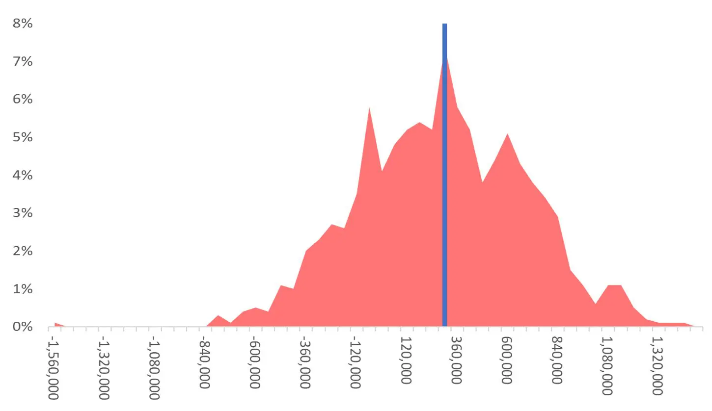
A simulation-based analysis might use 1,000 scenarios to generate distributions of hourly PPA payoffs and then aggregate those results by month and across the contract term.
The mean of the simulated outcomes provides an expected value under the model assumptions, while the distribution provides information about the range of possible outcomes.
This distinction is fundamental to PPA risk management – a PPA can have an attractive expected value while still carrying substantial downside risk.
For an introduction to this methodology, see What is Monte Carlo Simulation?
What the Risk Distribution Tells You
Looking only at expected PPA value can conceal the extent of the uncertainty around that value.
A simulation-based analysis can instead show:
- expected cash flow;
- favourable and adverse outcomes;
- the spread of possible results;
- how risk changes over time;
- seasonal concentrations of risk; and
- the effect of alternative hedging strategies.
For example, hourly simulated cash flows can be aggregated to monthly periods to show where risk is concentrated through the year. They can then be aggregated over the full PPA term to understand the overall distribution.
This allows the analysis to move from a question about value to a much broader question:
What could happen to the value and cash flows of this PPA under different market and generation outcomes?
That is the starting point for risk management.
Valuation and Risk Should Use the Same Underlying Framework
There is an important practical advantage to building valuation and risk analysis around the same underlying model: the simulated scenarios used to calculate expected PPA value can also be used to understand the distribution of outcomes and test potential hedges.
Rather than calculating a valuation using one set of assumptions and risk metrics using another, the same underlying representation can support both. This consistency becomes increasingly important when PPAs are aggregated into portfolios containing multiple renewable assets, markets and hedges.
The next step is to use that analysis to determine how the resulting exposures can be managed.
One-Sentence Takeaway
Valuing and assessing the risk of a renewable PPA requires modelling the interaction between power prices, generation, volume and time-dependent market characteristics to understand both its expected value and the range of possible outcomes.
Related Learning Resources
What is a Power Purchase Agreement (PPA)?
Understand how different PPA structures allocate price, volume and other risks between participants.
How to Hedge Power Purchase Agreements (PPAs)
Explore how the risks identified through PPA valuation can be managed using different hedging strategies.
What is Monte Carlo Simulation?
Learn how simulation is used to generate possible future market outcomes and support valuation and risk analysis.
Understand how stochastic models represent uncertainty in energy and commodity markets.