
 Search
Learning | Valuation & Pricing Analytics
What is a Trinomial Tree Model?
Introductory Summary
Many energy valuation problems require decisions to be made before future market prices are known.
Should gas be injected today or held for later? Is it better to exercise an option now or wait? Does operating an asset today reduce a more valuable opportunity tomorrow?
Questions like these cannot be answered by looking only at today’s market prices. They require a structured way to evaluate many possible future market outcomes and determine the best decision at every stage.
One of the most widely used techniques for solving these problems is the trinomial tree model.
Rather than attempting to predict exactly what will happen, a trinomial tree represents a range of possible future price paths. Then, using backward induction, practitioners can determine the optimal decision at every node.
Definition
A trinomial tree model is a numerical valuation technique that represents the evolution of many possible future price paths through a branching lattice. Each node represents one possible future market state generated by the calibrated model. Depending on the application, this may be price or inventory level for any time period.
At every node, a valuation algorithm determines the operating decision by maximising the expected value given the state of the node, subject to operational constraints.
At each time step, prices can move:
- upwards;
- remain approximately unchanged; or
- move downwards.
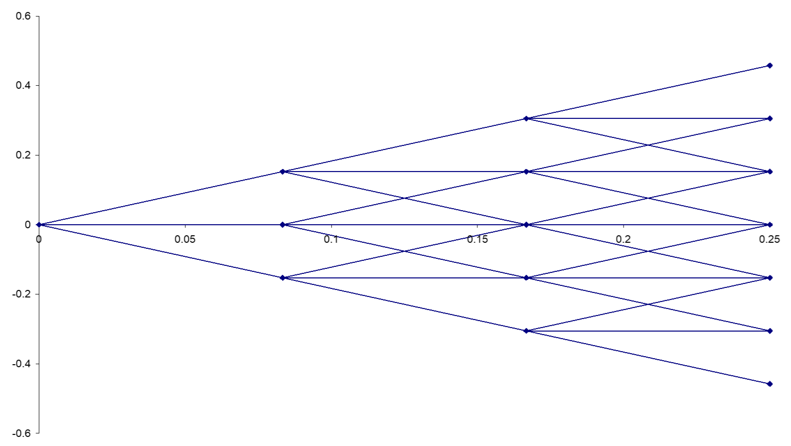
Each branch represents one possible future outcome. By evaluating decisions at every node in the tree, practitioners can determine the strategy that maximises value under uncertainty.
Unlike deterministic valuation methods, trinomial trees explicitly recognise that multiple future market outcomes are possible.
Why Three Branches?
The name “trinomial” comes from the fact that each node connects to three possible future states rather than two (as in binomial trees).
This additional branch provides greater flexibility in representing price behaviour and can improve numerical stability compared with simpler binomial approaches.
Although the mathematics behind the model can become sophisticated, the underlying concept remains intuitive: rather than assuming one future price, the model considers many possible prices that the market could reasonably reach through time.
How Is the Tree Constructed?
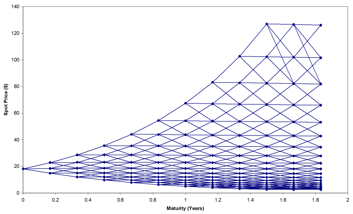
The branches in a trinomial tree are not chosen arbitrarily. They are generated from a calibrated stochastic price model that reflects current market conditions.
In practice, practitioners typically begin with today’s forward curve and calibrate the price model using observable market information such as volatility, mean reversion, and seasonality. For energy commodities, calibration may also incorporate characteristics such as volatility term structure and commodity-specific market behaviour.
The trinomial tree is constructed so that its possible future price paths are consistent with these market assumptions.
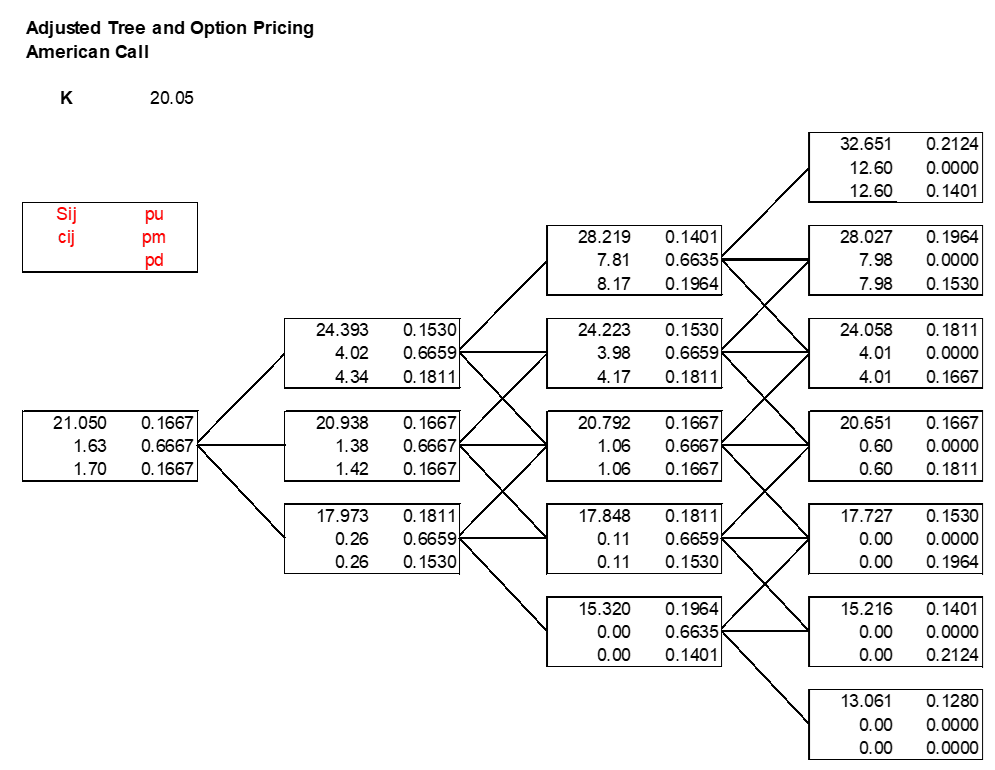
As the tree branches through time, each node represents one possible future market state (e.g. price) that could occur under the calibrated model. Backward induction is then used to determine the optimal decision at every node.
How Trinomial Trees Support Valuation
A trinomial tree does far more than simulate future prices – its real strength is helping determine the best decision at every possible future state. For example, when valuing a gas storage facility, the operator has three choices at each decision point:
- inject gas;
- withdraw gas; or
- wait.
Each choice changes the amount of gas remaining in storage and therefore affects the opportunities available in future periods.
The trinomial tree evaluates these alternatives across the entire network of possible future states (e.g. prices) to determine which decision creates the greatest overall value.
Rather than asking, “What is the best decision today?”, the model asks:
“What would the optimal decision be if prices reached this point in the future?”
It repeats this process for every possible state represented in the tree.
For example, imagine a gas storage asset today with three possible price outcomes next month: low, medium, and high. At each outcome, the operator decides whether to inject, withdraw, or wait. The model then looks further ahead, considering the value created by each possible future decision. By repeating this process backwards through every possible state, the model identifies the strategy that produces the highest value today.
Backward Induction
One of the defining characteristics of trinomial tree valuation is that they work backwards.
The model begins at the final period of the analysis, where the remaining value of the asset can be calculated directly.
It then sweeps backwards through the tree, evaluating every earlier decision by considering both:
- the immediate cashflow generated; and
- the value of preserving future operating flexibility.
This process, known as backward induction, continues until the valuation reaches today’s market conditions.
The resulting value reflects the optimal decisions throughout the entire life of the asset rather than a single operating strategy.
Where Are Trinomial Trees Used?
Trinomial tree models are widely used wherever future decisions depend on uncertain market prices.
Common applications include:
- gas storage valuation;
- swing contract valuation;
- tolling agreement valuation;
- energy option pricing;
- physical asset optimisation; and
- structured energy contracts.
In each case, the model helps identify how flexibility contributes to value.
Trinomial Trees Versus Monte Carlo simulation
Trinomial trees are one of several techniques used to solve stochastic valuation problems. Another common approach is Monte Carlo simulation. While both methods model uncertainty, they do so differently.
A trinomial tree evaluates decisions across a structured network of possible future market states. Monte Carlo simulation generates many individual price paths and optimises decisions along each simulated scenario.
| Trinomial Tree | Monte Carlo | |
|---|---|---|
| Future uncertainty | Discrete lattice of states | Many simulated paths |
| Decision optimisation | Naturally supports backward induction | Often requires additional optimisation techniques |
| Transparency | High | Often lower |
| High-dimensional problems | Can become computationally demanding | Often more scalable |
Both approaches are widely used in energy markets, with the most appropriate technique depending on the characteristics of the asset, the pricing model, and the analytical problem being solved.
Common Pitfalls and Misconceptions
Trinomial Trees Predict Future Prices
They do not. A trinomial tree represents a range of possible future market outcomes rather than attempting to forecast which one will occur.
More Branches Always Produce Better Results
Increasing the complexity of a tree does not automatically improve valuation accuracy. The quality of the underlying price model, calibration, and market assumptions typically has a much greater influence on the reliability of the results.
Trinomial Trees Produce a Single Strategy
A trinomial tree does not produce a single fixed operating schedule. Instead, it produces a dynamic decision strategy that adapts as market conditions evolve.
Trinomial Trees Are Only Used for Options
Although widely associated with option pricing, trinomial trees are also used to value physical assets and contracts whose value depends on future operational decisions. Gas storage is one prominent example.
How Trinomial Tree Models Are Applied in Practice
Trinomial trees are rarely used in isolation.
Practitioners first develop forward curves, calibrate stochastic price models, and define the physical or contractual constraints of the asset being analysed. The trinomial tree is then used to evaluate the optimal decisions across all possible future market states.
Maintaining these models can become increasingly complex as organisations expand across multiple commodities, assets, and market regions. Many organisations therefore use integrated analytics tools to support model calibration, tree construction, valuation, and governance.
Applications such as Lacima Trader can support practitioners by bringing together model calibration, tree construction, valuation, and governance within a consistent framework.
One-Sentence Takeaway
A trinomial tree model values assets with embedded flexibility by representing many possible future market outcomes and working backwards to determine the optimal decision at every stage.
Related Learning Resources
See how trinomial trees are used to determine optimal injection and withdrawal decisions when valuing gas storage assets.
What is Monte Carlo simulation?
Compare lattice-based valuation with simulation-based approaches for modelling uncertain future market prices.
Learn how stochastic price models provide the foundation for trinomial trees and other quantitative valuation methods.
How to Value Tolling Agreements
Explore another practical application of trinomial tree models for valuing assets with operational flexibility.