
 Search
Learning | Quantitative Modelling Concepts
What is a Single-Factor Model?
Introductory Summary
Many quantitative models begin with a simple question:
“How should market prices evolve through time?”
Rather than attempting to predict exactly where prices will go, quantitative models simulate many possible future price paths that reflect how markets are expected to behave.
A single-factor model is one of the simplest and most widely used approaches for doing this.
It assumes that a single underlying stochastic process drives the evolution of prices through time. Depending on the assumptions made about that process, the model can represent behaviours such as steady growth, mean reversion, or sudden price jumps.
Despite their relative simplicity, single-factor models remain widely used throughout energy and commodity markets because they often provide an effective balance between realism, transparency, and computational efficiency.
Definition
A single-factor model is a stochastic price model in which a single source of uncertainty drives the evolution of market prices over time.
Rather than assuming future prices are known, the model generates many possible price paths by allowing one underlying stochastic process to evolve through time.
Different assumptions about that process produce different types of single-factor models. For example, prices may:
- follow continuous random movements;
- gradually revert towards a long-term equilibrium level; or
- occasionally experience sudden jumps.
Although different single-factor models produce different types of price behaviour, they all share the same underlying principle: a single stochastic process drives the evolution of prices through time.
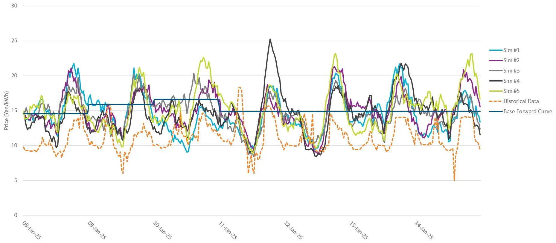
What Does the Single-Factor Represent?
The word factor refers to the underlying stochastic process that drives price movements. In a single-factor model, every future price is influenced by that one process.
For example, a model may assume that prices fluctuate randomly around today’s market expectations while gradually reverting towards an equilibrium level. Alternatively, it may assume prices follow continuous random movements without any tendency to revert.
The choice of stochastic process determines how prices behave throughout the simulation.
Importantly, the single-factor does not mean only one market price is being modelled. Instead, it means one underlying source of uncertainty governs the evolution of that market. It is this underlying stochastic process, not the price itself, that is referred to as the model’s single-factor.
Common Single-Factor Price Models
The behaviour of a single-factor model depends on the assumptions made about its underlying stochastic process. Common examples include:
Geometric Brownian Motion (GMB)
Geometric Brownian Motion assumes prices evolve continuously with constant volatility and no tendency to return towards previous levels.
It forms the foundation of many classical financial pricing models and remains widely used where persistent price trends are considered appropriate.
Mean-Reverting Models
Many energy and commodity prices exhibit mean-reverting behaviour. Mean-reverting single-factor models assume prices tend to move back towards a longer-term equilibrium level at a mean reverting rate.
This often provides a more realistic representation of many physical commodity markets than models that assume prices simply drift indefinitely.
Mean-Reverting Jump Diffusion Models (MRJD)
Some commodity markets occasionally experience sudden price movements caused by unexpected events such as supply disruptions, extreme weather, or infrastructure failures. A Mean Reversion Jump Diffusion model combines gradual mean-reverting price behaviour with the possibility of these occasional price jumps.
Between jumps, prices evolve according to the normal mean-reverting process. When a jump occurs, prices can move sharply before subsequently reverting towards their longer-term equilibrium. This allows the model to represent both the day-to-day behaviour of commodity prices and the occasional extreme events observed in real markets.
We explore how MRJD models work in more detail in the What is Mean Reversion Jump Diffusion (MRJD)? article.
Why Single-Factor Models Are Widely Used
Single-factor models remain popular because they capture many important characteristics of market behaviour while remaining relatively efficient to calibrate and simulate.
They are commonly used for:
- derivative valuation;
- risk analysis;
- Monte Carlo simulation;
- asset valuation;
- portfolio modelling; and
- investment analysis.
Because only one stochastic process needs to be modelled, they are generally easier to understand, calibrate, and maintain than more complex modelling approaches.
For many applications, they provide an appropriate balance between model realism and computational efficiency.
When Multi-Factor Models Become Useful
While single-factor models are capable of producing realistic price simulations, they also have limitations.
Because a single stochastic process drives the entire market, the resulting forward curve tends to move in relatively simple ways.
For many assets, this is entirely appropriate. However, some valuation problems depend on changes in the relationships between different delivery periods rather than changes in the overall market level.
Gas storage is a good example of this. The value of a storage facility often depends on how seasonal price spreads evolve through time rather than whether the entire forward curve simply moves higher or lower.
Representing these more complex market dynamics often requires additional stochastic factors, and a reason multi-factor models are frequently used for more sophisticated energy valuation problems.
Single-Factor Versus Multi-Factor Models
Both modelling approaches simulate uncertain future prices. The difference lies in how many independent sources of uncertainty drive those simulations.
A single-factor model assumes one stochastic process governs market behaviour.
A multi-factor model combines several independent stochastic processes, allowing different parts of the forward curve, or different aspects of market behaviour, to evolve separately.
Choosing between them depends on the asset being valued, the characteristics of the market, and the objectives of the analysis.
Common Pitfalls and Misconceptions
Single-Factor Means Only One Price Is Modelled
A single-factor model may be used to simulate an entire market. The term refers to the number of stochastic processes driving price evolution, not the number of prices being represented.
Single-Factor Models Are Too Simple for Real Markets
Not necessarily. Many widely used quantitative valuation models are single-factor models because they provide an effective balance between realism, transparency, and computational efficiency. The appropriate choice of model depends on the complexity of the problem being solved, and the objectives of the analysis.
Multi-Factor Models Always Produce Better Results
Additional factors allow more complex market behaviour to be represented, but they also introduce greater calibration requirements and model complexity. More sophisticated models are only beneficial when that additional complexity improves the quality of the analysis.
How Single-Factor Models Are Applied in Practice
In practice, a single-factor model is rarely used in isolation.
Practitioners typically combine it with forward curves, volatility assumptions, mean reversion, calibration techniques, and Monte Carlo simulation to create a coherent representation of future market behaviour.
For many organisations, the challenge is not simply selecting an appropriate price model, but ensuring that the same market assumptions are used consistently across valuation, optimisation, trading, and enterprise risk management.
Integrated analytics platforms such as Lacima Analytics enable organisations to maintain a common market model across these analytical disciplines, improving consistency, governance, transparency, and auditability while reducing the need to manage separate modelling frameworks.
One-Sentence Takeaway
A single-factor model uses one underlying stochastic process to simulate future price behaviour, providing an efficient and widely used foundation for valuation, simulation, and risk analysis across energy and commodity markets.
Related Learning Resources
Discover how multi-factor models extend single-factor approaches by allowing several independent sources of uncertainty to influence market behaviour.
Learn why many energy prices tend to move back towards longer-term equilibrium levels and how this behaviour is incorporated into single-factor price models.
What is Mean Reversion Jump Diffusion (MRJD)?
Discover how MRJD models extend standard mean-reverting models by incorporating occasional price jumps caused by unexpected market events.
Explore how stochastic models generate realistic future price scenarios for valuation and risk analysis.