
 Search
Learning | Quantitative Modelling Concepts
What is a Simulation Path?
Introductory Summary
In quantitative energy modelling, practitioners often talk about running thousands of simulations. But what is actually being simulated?
The answer is usually a simulation path – one possible future trajectory for prices, rates, or other market variables generated by a stochastic model.
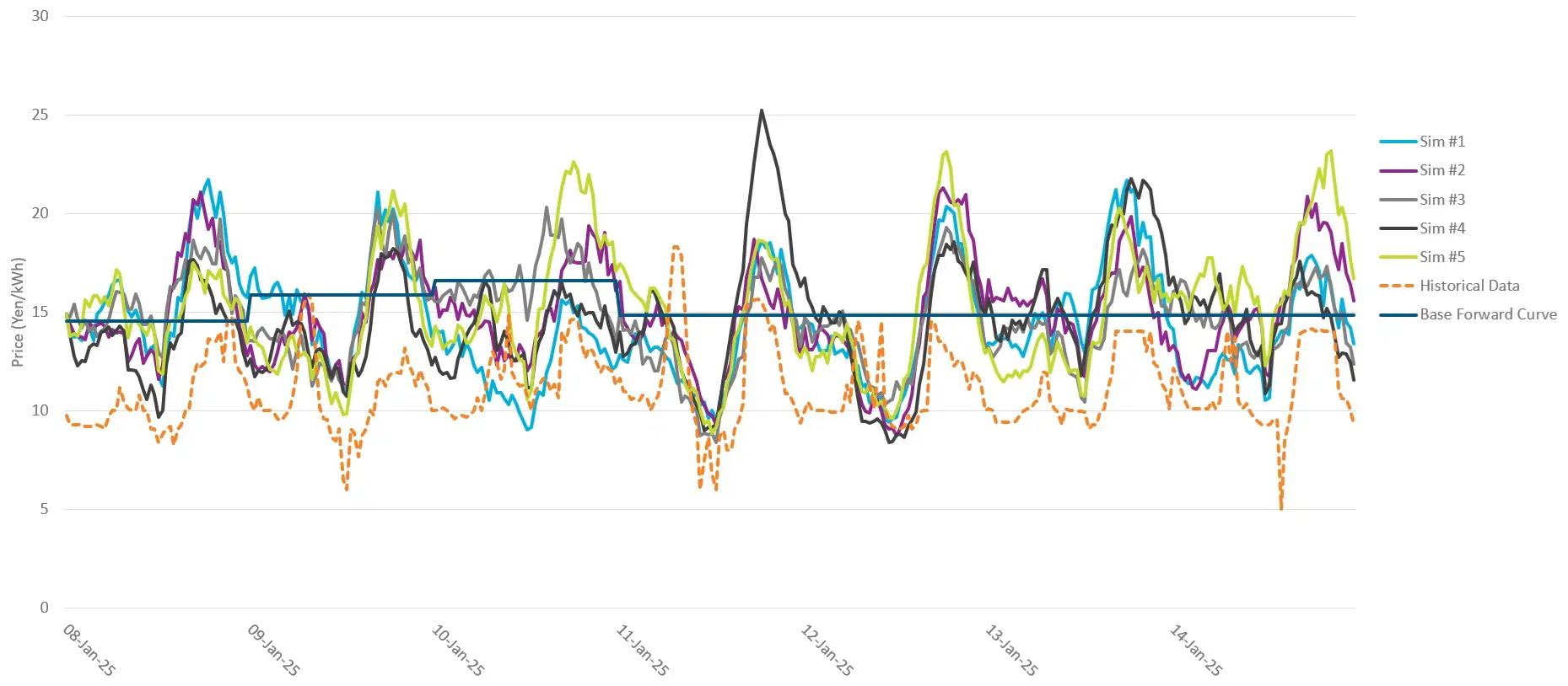
For example, an electricity price model might produce 10,000 different future price paths. Each path represents one possible way the market could evolve over time. No individual path is expected to be the “correct” forecast. Instead, the collection of paths represents the range of outcomes that the model considers possible.
This idea sits at the heart of Monte Carlo simulation, Value at Risk (VaR), option valuation, storage valuation, and many other forms of quantitative energy analytics.
Definition
A simulation path is one possible future sequence of values generated by a stochastic model.
Starting from today’s market conditions, the model evolves prices forward through time according to its calibrated assumptions about volatility, mean reversion, correlations, jumps, and other sources of uncertainty.
For example, a single gas price path might look like this:
| Date | Simulated Gas Price |
|---|---|
| Today | $12 |
| 1 Month | $13 |
| 2 Months | $11 |
| 3 Months | $15 |
| 4 Months | $14 |
Another simulation path would produce a different sequence of prices.
Both are possible futures generated from the same underlying model.
A Simulation Path Is Not a Forecast
When a model generates a simulation path, it is not predicting exactly what will happen. Instead, it is generating one realisation of the stochastic process.
If a model is run 10,000 times, it will produce 10,000 different paths. Some may show rising prices, some falling prices, and others highly volatile behaviour.
The purpose is not to identify the single “right” future. In fact, if a model generates thousands of different simulation paths, they cannot all represent what will actually happen. Instead, each path represents one possible future, and together they help quantify the range and likelihood of possible market outcomes.
How Simulation Paths Are Generated
Most quantitative energy models begin with a stochastic price model such as:
The model then uses random sampling to generate future movements through time.
At each time step, the process produces a new simulated value based on the model’s assumptions and the random shocks generated for that simulation.
Repeating this process step-by-step creates a complete future path.
Why Thousands of Paths Are Used
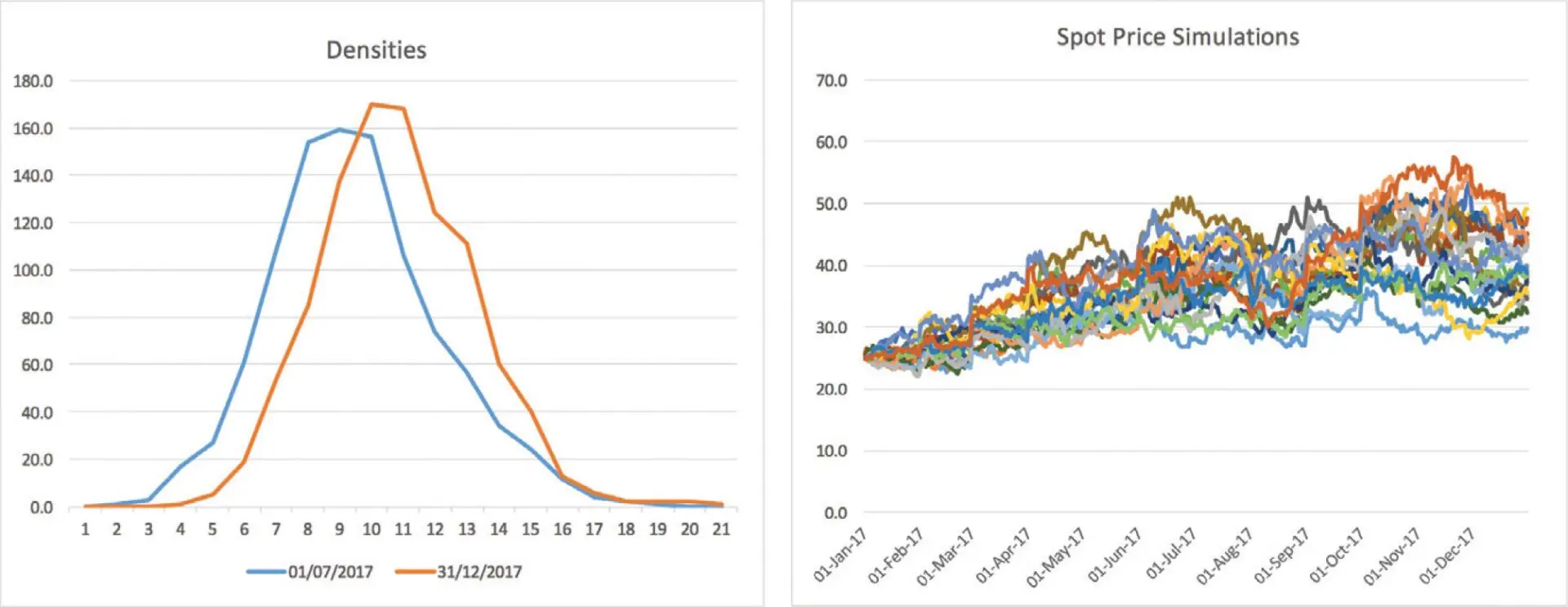
One simulation path provides only one possible outcome. To estimate expected values and risks, practitioners usually generate many paths.
For example:
- 1 path = one possible future
- 1,000 paths = a broad range of possible futures
- 10,000+ paths = a richer estimate of value and risk
Monte Carlo simulation works by analysing the results across all simulated paths. For instance, when valuing a gas storage facility, the optimisation is performed independently along every simulated path. The resulting cashflows are then analysed collectively to estimate the asset’s expected value and risk.
Why Simulation Paths Matter
Many quantitative techniques depend on evaluating more than one possible future.
A simulation path represents one possible evolution of future market conditions. By generating and analysing thousands of these paths, practitioners can estimate expected values, quantify risk, evaluate uncertainty, and better understand how different market conditions may influence commercial decisions.
This ability to analyse many possible futures is one of the defining strengths of modern quantitative energy modelling.
Common Pitfalls and Misconceptions
More Paths Guarantee Better Results
Not necessarily. The quality of the underlying model and its calibration is usually more important than simply increasing the number of simulations.
Practitioners typically choose enough simulation paths for the results to become sufficiently stable for the purpose of the analysis. Beyond that point, generating additional paths may increase computation time while providing little additional insight.
All Simulation Paths Are Equally Likely
The model assigns probabilities implicitly through its stochastic assumptions. Some regions of the simulated outcome distribution may be much more likely than others.
The Highest-Probability Path Is the Forecast
A simulation path is not intended to be a forecast. It is one possible future generated by the model.
How Simulation Paths Are Used in Practice
Once a set of simulation paths has been generated, the same paths can support many different analytical activities. For example, an organisation may use the identical set of simulated market scenarios to:
- value storage assets;
- price structured contracts;
- calculate Value at Risk (VaR);
- perform stress testing;
- evaluate hedging strategies; and
- analyse portfolio performance under changing market conditions.
Using a common set of simulation paths across these activities helps ensure that different analytical teams are working from the same representation of future market uncertainty.
Integrated analytics applications such as Lacima Analytics enable organisations to generate, manage, and reuse simulation paths across multiple valuation, optimisation, and risk management processes within a single analytical framework.
One-Sentence Takeaway
A simulation path is one possible future trajectory generated by a stochastic model, and Monte Carlo analysis uses many such paths to estimate values, risks, and portfolio behaviour under uncertainty.
Related Learning Resources
Learn how stochastic models generate possible future market outcomes.
What is Monte Carlo simulation?
See how thousands of simulation paths are combined to estimate values and risks.
Understand one of the most common stochastic processes used to generate simulation paths.
Explore how multiple sources of market uncertainty can be simulated together.