
 Search
Learning | Quantitative Modelling Concepts
How to Perform Monte Carlo Simulation
Introductory Summary
Monte Carlo simulation is one of the most widely used techniques in quantitative energy and commodity analytics.
Rather than attempting to predict a single future outcome, it evaluates thousands of possible market scenarios, allowing practitioners to estimate asset values, quantify risk, and optimise operational decisions under uncertainty.
Each scenario represents one possible evolution of uncertain market variables over time. In energy markets these variables most commonly include commodity prices, but may also incorporate other stochastic market factors depending on the model being used.
The simulated market scenarios then provide the foundation for valuation, optimisation and risk analysis.
This article explains how to perform Monte Carlo simulation. For a detailed explanation of the underlying principles of Monte Carlo simulation, see What is Monte Carlo simulation?
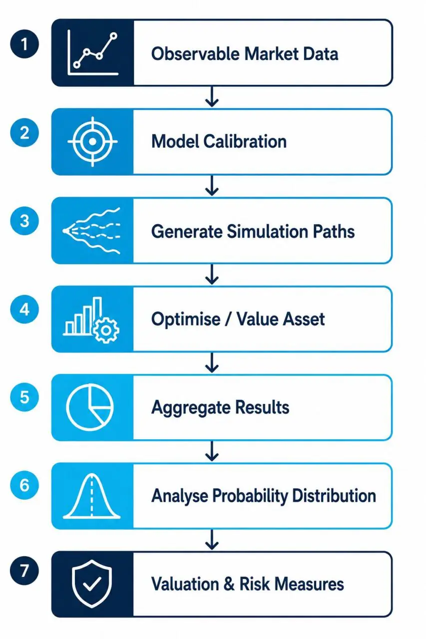
Step 1: Build and Calibrate a Market Model
Every Monte Carlo simulation begins with a market model that describes how the market being analysed may evolve through time.
Depending on the characteristics of the market being analysed, the model may incorporate behaviours such as:
- mean reversion;
- stochastic volatility;
- jump behaviour;
- correlations between market variables; or
- multiple stochastic factors.
The model must then be calibrated using observable market information. Depending on the application, practitioners may estimate model parameters from:
- historical spot prices;
- forward curves;
- option market prices;
- implied volatilities;
- observed market correlations; and
- other relevant market information.
Calibration transforms a mathematical model into one that represents current market behaviour. Every simulation generated afterwards depends on the quality of this calibration.
Step 2: Generate Simulation Paths
Once the market model has been calibrated, it can generate possible future market scenarios.
Starting from today’s market conditions, the model progresses forward one time step at a time, using random sampling together with the calibrated model assumptions to determine how the simulated market evolves.
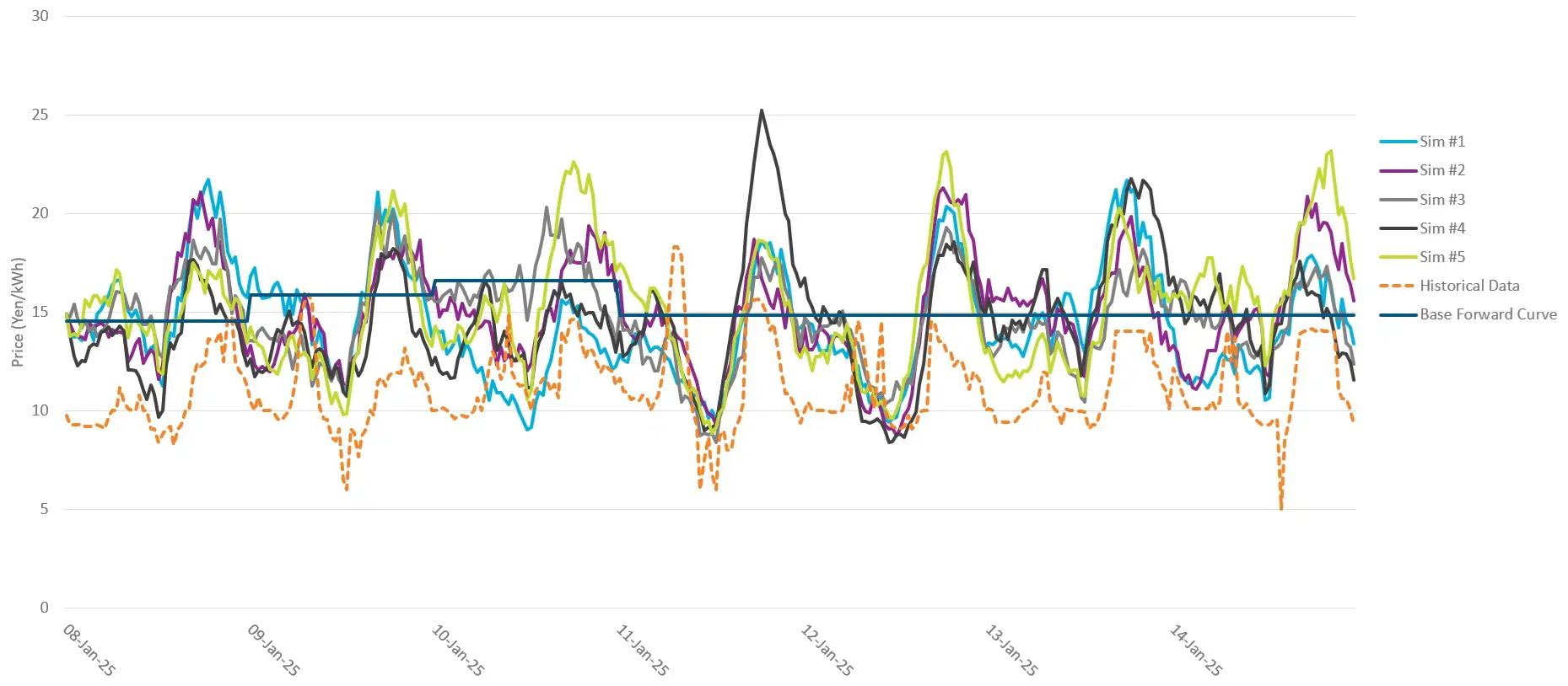
Repeating this process many times produces a large collection of simulation paths.
No individual path is expected to represent the future exactly. Instead, together they describe the range of outcomes that the model considers possible.
Step 3: Evaluate Each Simulation
Generating simulation paths is only the beginning. The real value of Monte Carlo simulation comes from analysing what happens along every simulated future.
Depending on the application, practitioners may:
- value energy options;
- optimise gas storage operations;
- optimise grid-scale battery storage;
- value swing contracts;
- analyse structured commodity contracts; or
- evaluate portfolio cashflows.
For operational assets, every simulation path may produce a different sequence of operating decisions because optimal decisions depend on both market prices and the evolving state of the asset.
For example, a gas storage facility may inject gas under one simulated price path, withdraw gas under another, and remain idle under a third.
Each simulation therefore produces both different market outcomes and different operational decisions.
Step 4: Aggregate the Results
After every simulation has been evaluated, the individual results are aggregated into a statistical distribution.
Rather than focusing on any individual simulation path, practitioners analyse the distribution of outcomes across the entire simulation set.
From this distribution they can estimate:
- expected asset value;
- Value at Risk (VaR);
- downside risk;
- upside potential;
- confidence intervals;
- probability distributions; and
- other portfolio risk measures.
Step 5: Analyse the Results
Once all simulation paths have been analysed, practitioners examine the distribution of outcomes rather than focusing solely on the average value.
Analysing the distribution of outcomes allows decision-makers to understand not only what may happen, but also how likely different outcomes may be.
Depending on the objective of the analysis, they may consider:
- the expected (average) value;
- downside outcomes such as the 1st or 5th percentile;
- upside outcomes such as the 95th or 99th percentile;
- the spread of results; and
- the probability of particular commercial outcomes occurring.
For example, while the average valuation may represent the expected outcome, the lower percentiles help quantify downside risk, while the upper percentiles illustrate the potential upside if market conditions prove favourable.
Examining the full distribution enables organisations to understand both expected performance and the range of uncertainty surrounding that expectation.
Why Thousands of Simulations Are Needed
One simulation path represents only one possible future.
Reliable valuation and risk analysis require many possible futures to be considered.
As the number of simulation paths increases, estimated values and risk measures generally become more stable.
Practitioners therefore select enough simulations for the results to converge to an acceptable level of stability for the purpose of the analysis. Beyond that point, generating additional simulations may increase computation time while providing relatively little additional insight.
Common Pitfalls and Misconceptions
Monte Carlo simulation Predicts Future Prices
Monte Carlo simulation generates many plausible future market scenarios. It does not attempt to identify exactly what will happen.
More Simulations Always Produce Better Results
Not necessarily. Once the results have stabilised, improving the market model or its calibration will often deliver greater benefits than simply generating more simulation paths.
Monte Carlo simulation Is Only Used for Option Pricing
Monte Carlo simulation supports a wide range of applications including physical asset valuation, storage optimisation, structured contract valuation, portfolio risk measurement, investment analysis, and enterprise risk management.
How Monte Carlo simulation Is Applied in Practice
Organisations rarely build separate Monte Carlo models for individual analytical tasks.
Instead, a single calibrated market model is often reused across multiple activities, allowing the same representation of future market behaviour to support valuation, optimisation, portfolio risk measurement, investment analysis, and commercial decision-making.
This shared approach helps ensure different teams are working from a consistent representation of future market behaviour, improving transparency, governance, and confidence in analytical results.
Applications such as Lacima Analytics support this workflow by enabling organisations to build, calibrate, govern, and reuse Monte Carlo simulation models across valuation, optimisation, trading, commercial, finance, and risk management within a common analytical environment.
One-Sentence Takeaway
Performing Monte Carlo simulation involves building and calibrating an appropriate market model, generating many possible future market scenarios, evaluating assets under each scenario, and aggregating the results to estimate value and quantify risk.
Related Learning Resources
What is Monte Carlo simulation?
Learn the principles behind Monte Carlo simulation and why it is widely used for valuation and risk analysis.
Explore how individual simulation paths are generated and why thousands of paths are analysed together.
Understand why accurate model calibration is essential before performing Monte Carlo simulation.
What is an Energy Trading and Risk Management (ETRM) System?
Understand what ETRM systems do, where their limitations lie, and why organisations complement them with specialist valuation and risk analytics.