
 Search
Learning | Quantitative Modelling Concepts
How to Model Energy Price Volatility
Introductory Summary
Volatility is one of the defining characteristics of energy markets.
Electricity prices can experience sudden and significant spikes. Gas prices may remain relatively stable for extended periods before responding rapidly to supply disruptions or changing weather conditions. Carbon markets, LNG markets, and oil markets each exhibit their own distinctive patterns of price variability.
Capturing this behaviour accurately is one of the primary objectives of quantitative energy modelling.
Rather than treating volatility as a single number, practitioners develop market models that reproduce the way volatility behaves in practice. Depending on the market, this may involve representing changing volatility, price jumps, mean reversion, or several of these characteristics together.
This article explains the practical process of modelling energy price volatility. For a more detailed explanation of volatility itself, see What is a Volatility Function?
Why Volatility Modelling Matters
Many quantitative energy applications depend on how prices fluctuate through time rather than simply where prices may end up. For example, volatility influences:
- option values;
- gas storage valuation;
- battery optimisation;
- portfolio risk;
- Value at Risk (VaR);
- hedge performance; and
- investment decisions.
If volatility is represented unrealistically, the resulting valuation or risk analysis may not accurately reflect the commercial opportunities and risks associated with the asset being analysed.
Choosing an appropriate volatility model is therefore an important part of building a reliable market model.
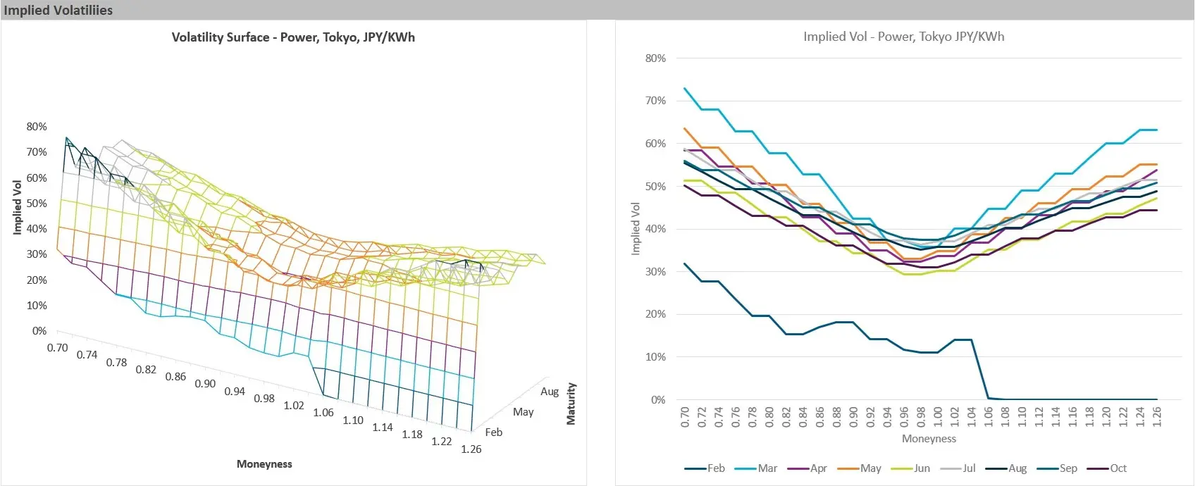
Step 1: Understand How the Market Behaves
Before selecting a modelling framework, practitioners first consider the characteristics of the market itself. Important questions include:
- Do prices tend to revert towards a long-term equilibrium?
- Do periods of high volatility alternate with quieter periods?
- Are sudden price spikes common?
- Do different commodities influence one another?
- Does volatility vary across different delivery periods?
Step 2: Select an Appropriate Stochastic Model
Different markets often require different modelling approaches because their price behaviour can vary significantly. Once the important market characteristics have been identified, an appropriate stochastic modelling framework can be selected.
Depending on the application, practitioners may use:
- mean reversion models;
- mean reversion jump diffusion (MRJD) models;
- stochastic volatility models;
- single-factor models; or
- multi-factor models.
Each framework represents market behaviour differently.
For example, a mean reversion model may be appropriate where prices fluctuate around a longer-term equilibrium, while a Mean Reversion Jump Diffusion (MRJD) model can additionally represent the occasional extreme price movements frequently observed in electricity and gas markets.
The objective is not to build the most complex model possible, but to select one that captures the important characteristics of the market being analysed.
Step 3: Calibrate the Model
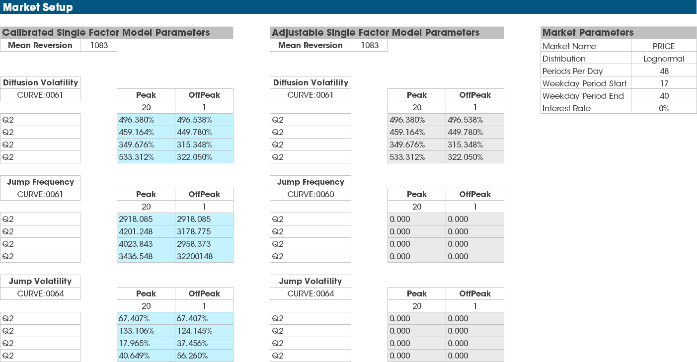
After selecting the modelling framework, its parameters must be calibrated using observable market information. Depending on the application, calibration may use:
- historical spot prices;
- forward curves;
- option market prices;
- implied volatilities;
- observed market correlations; and
- other relevant market information.
These data sources provide the evidence used to estimate model parameters such as volatility, mean reversion speed, jump behaviour, or correlations.
Calibration transforms a theoretical stochastic model into one that reflects current market behaviour.
Step 4: Validate the Model
Calibration alone is not sufficient. Practitioners typically validate the calibrated model to confirm that it reproduces the market characteristics it was designed to represent.
For example, they may assess whether simulated prices exhibit:
- realistic levels of volatility;
- appropriate mean-reverting behaviour;
- plausible price spikes;
- representative correlations; and
- statistical characteristics consistent with observed markets.
Validation provides confidence that the model is suitable for its intended analytical purpose before it is used for valuation or risk analysis.
Step 5: Apply the Model
Once validated, the market model can support a wide range of analytical applications. For example, the same calibrated volatility model may be used to:
- perform Monte Carlo simulation;
- value physical assets;
- optimise storage operations;
- value structured commodity contracts;
- measure portfolio risk;
- calculate Value at Risk (VaR); and
- evaluate investment opportunities.
Using a common market model across these activities helps maintain consistency throughout the organisation’s analytical processes.
Common Pitfalls and Misconceptions
Higher Volatility Always Means Higher Risk
Not necessarily. Greater volatility generally increases uncertainty, but its commercial impact depends on the nature of the asset or contract. For example, higher volatility may increase the value of many options because it creates more opportunities for favourable outcomes.
Every Market Can Be Modelled the Same Way
Different energy markets often exhibit very different behaviour.
A modelling framework that performs well for one commodity or region may not provide an appropriate representation of another.
A More Complex Model Is Always Better
Not necessarily. Additional complexity is only valuable when it improves the model’s ability to represent meaningful market behaviour. Simpler models are often preferable when they adequately support the analytical objective.
How Volatility Modelling Is Applied in Practice
Volatility modelling is rarely undertaken for a single valuation exercise. Instead, organisations often develop and govern shared market models that represent volatility consistently across trading, commercial, finance, and risk management activities.
This allows the same calibrated representation of market behaviour to support asset valuation, optimisation, portfolio risk measurement, investment analysis, and stress testing, reducing the risk of different business functions working from inconsistent market assumptions.
Applications such as Lacima Analytics support this approach by enabling organisations to calibrate, validate, govern, and reuse volatility models across multiple analytical disciplines within a common analytical environment.
One-Sentence Takeaway
Modelling energy price volatility involves selecting an appropriate stochastic modelling framework, calibrating it to observable market behaviour, validating its performance, and applying it consistently across valuation, optimisation, simulation, and risk analysis.
Related Learning Resources
Understand why accurate calibration is essential for reliable volatility modelling.
How to Perform Monte Carlo simulation in Energy Markets
See how calibrated volatility models are used to generate simulation paths for valuation and risk analysis.
What is an Energy Trading and Risk Management (ETRM) System?
Understand what ETRM systems do, where their limitations lie, and why organisations complement them with specialist valuation and risk analytics.
Learn how stochastic models generate possible future market outcomes.